|
Simple coil design methods that work
The fin-and-tube heat exchanger is probably the most common piece of equipment found in any air-conditioning installation. These heat exchangers are typically referred to as coils and are designated by the fluids in the tube. So, a chilled water coil is a fin-and-tube heat exchanger used for cooling air where the coolant is chilled water and the direct expansion coil is a fin-and-tube evaporator found in a vapour compression cycle. These two coil types are primarily used to cool air. In most cases, the temperature of the coolant at the coil inlet is in the order of 6 ºC and at typical air-conditioning temperatures, this would result in a coil surface temperature that is below the dew point of the air being cooled. The consequence of this is that there will be condensation on the coil surface and this condensate is clearly evident by the water flowing out of the drain pans of many installations. Methods to design and select heating coils are based on an overall heat transfer coefficient multiplied by the appropriate temperature difference. In cooling coils where there is condensation, the temperature difference is not the correct driving force since the latent heat of condensation is not accounted for. There have been different ways of dealing with this shortfall. These include the introduction of a sensible heat factor to modify the outside film coefficient, use of a log mean enthalpy difference and the effectiveness method based on a saturation specific heat. In this paper, we develop the equations and by simulation, illustrate the validity of the effectiveness method for solving wet surface cooling coils.
The conventional LMTD methodThe LMTD method is a well-known way of calculating a heat exchanger size. The idea is that the heat exchanger has a pre-defined heat transfer coefficient and that the driving force for heat flow is the temperature difference. Q = Uo Ao dt This is the same equation as would be used to calculate heat flow across a wall of known conductivity. The difference in a heat exchanger is that the temperature of the fluids changes significantly. Without going into the details here, it can be shown that the effective temperature difference for parallel and counter flow configurations can be calculated from the following equation. dt = (dti – dto) / ln (dti / dto) Hence the name, log mean temperature difference. In the case of a cross flow and multi-pass configurations, you would have to apply an additional correction factor. The problem with the LMTD method is that the fluid leaving conditions must be known in order to calculate the duty. Clearly, if you know the leaving conditions, then you already know the duty. This makes the performance calculation of an existing coil an iterative process. A difficulty that often appears during the course of a simulation is that successive estimates of the leaving fluid temperatures could result in a negative (dti / dto) and consequently a program crash.
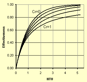
e-Ntu methodThe e-Ntu method is based on the concept of an efficiency rating and is defined by the following equation. Q = e Qmax The maximum duty can be easily determined when you realize that the fluid with the lowest capacity rate Cmin will have the largest temperature difference. In an ideal heat exchanger, that is one with an efficiency of 100%, the fluid with the lowest capacity rate will experience the maximum possible temperature difference or the inlet temperature difference (ITD). ITD = thi – tci Qmax = Cmin ITD Now you can see the benefit of this method since it is based on inlet conditions only and the actual duty is bounded between 0 and Qmax or in other words, an effectiveness of 0 to 1. It turns out that the effectiveness can be derived for many of the common heat exchanger configurations. These are well known and published in most heat transfer books in the form shown in Figure 1. Figure 1. Effectiveness of a single pass counter-flow heat-exchanger
For a counter-flow configuration, the effectiveness can be calculated from the following equation, e = (1 – e –Ntu (1-Cr) ) / (1 – Cr e –Ntu (1-Cr) ) where the number of transfer units Ntu = Uo Ao/Cmin and the capacity ratio Cr = Cmin/Cmax
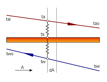
Step-by-step simulationIn developing theories, we often make assumptions to simplify the result so it would be instructive to be able to make a practical comparison. If we break the heat exchanger into a number of small pieces, it would be possible to calculate the heat flow at each step without making any assumptions. Figure 2. Thermal model of dry cooling
At each step, from tai to tao in the thermal model shown in Figure 2, the outside and inside heat transfer relationships need to be reconciled dq = ho dAo (ta – ts) dq = Ui dAi (ts – tw) This allows the determination of the surface temperature, ts and consequently the differential heat flow dq that is summed to get the total heat flow. Looking at each fluid in turn, it is also possible to calculate the next temperature from dq = Ca dta and dq = Cw dtw In a counter flow arrangement, this is an iterative process since in the direction of the airflow we would have to start with a guess of the leaving water temperature. At the end of the cycle, the water inlet temperature must be compared with the known inlet water temperature and the initial guess revised until a solution has been found.
Dealing with condensationWhen the surface temperature falls below the dew point temperature of the air, there will be condensation. This complicates matters since the energy balance must now include the mass and energy flow of the condensate. This means that there are two energy equations on the air-side, accounting for sensible and latent heat. dqs = ho dAo (ta – ts) dql = hd dAo (Wa – Ws) hfg By summing these two equations, it can be shown that the total energy can be approximated in terms of an enthalpy potential. dqt = hd dAo (ha – hs) So, the potential for heat transfer is the enthalpy difference between the moist air and the enthalpy of saturated air at the surface temperature.
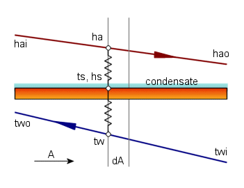
Simulation of a cooling coil with condensationBy incorporating the enthalpy potential, we can now simulate the performance of a cooling coil with condensate. In Figure 3, we see that the surface is wet and therefore the enthalpy at the surface is that of saturation air at the surface temperature. Figure 3. Thermal model of wet cooling coil
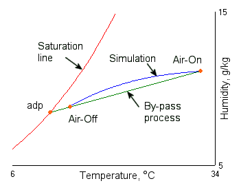
In addition to the heat transfer, we can calculate the condensate flow from dm = hd dAo (Wa – Ws) and consequently the absolute humidity at the next step as the simulation proceeds. The psychrometric chart in figure 4 shows the actual simulated process and the by-pass model based on the Ntu method. Figure 4. Psychrometric chart showing simulation and Ntu model
Notice that I have chosen a water supply temperature that would ensure a fully wet coil. In practice, it is possible that the inlet coil surface temperature could be above the air dew point and the coil would start out dry. As the air moves through the coil, it would be exposed to a lower temperature and condensation would start somewhere in the coil. This complicates the Ntu process since the coil should really be split into a dry and wet portion. The results of a wet coil model are however close enough not to warrant this precaution. In the case of a partially wet coil, Braun et al have suggested using the average between the wet and dry duties.
Problems with the LMTD methodThe problem with the LMTD method is that it is only valid for single-phase heat transfer. The reason is that the driving force is based on a temperature difference. If your instinct was to consider a log mean enthalpy difference, you would be on the right track. In fact, there are many references that adopt this approach (Kuehn et al ). Another approach would be to apply a sensible heat correction factor to the outside film coefficient. This would give an overall coefficient 1/Uo = SHR/ho + B/Ui. This modification is based on the air-side duty of dql = (ho Ao dt)/SHR and gives good correlation but does not always behave well numerically.
Validity of e-NtuIf the LMTD method doesn’t work for a wet coil, why then should the e-Ntu method be any different? The reason that it does work is that the maximum duty is based on the correct driving force. In a wet coil, the maximum duty is Qmax = ma (hai – hswi) And the duty can be calculated directly from Q = e Qmax For a wet coil, we now need to find a way to calculate the effectiveness. If we equate the air and water-side duties ma (hai - hao) = mw Cpw (twi - two) and define a saturation specific heat as Cs = (hswi - hswo) /(twi - two), we can replace the water temperature difference and re-arrange the energy balance equation into a form that looks similar to the dry case. ma Cs (hai - hao) = mw Cpw (hswi - hswo) By similarity, we can define the air capacity rate as Ca = ma Cs and adopt the effectiveness method in the same way that we did with a dry process. The definition of the saturation specific heat has given us this advantage.
Reference e-Ntu MethodThe conventional e-Ntu method does work well, but is difficult to program since you need to determine the maximum and minimum capacity rate in order to calculate the capacity ratio. In addition, you must base the maximum duty on the fluid with the minimum capacity rate. So, if for example you change the flow rate of the air, the relative positions of the fluids need to be revised. A possibility is to define a reference fluid and use this instead of the minimum capacity rate fluid. If we select air to be the reference fluid, the duty can be calculated from the following. Q = e Qair Qdry = ma Cpa (tai - twi) Qwet = ma (hai - hswi) e = (1 – e –Ntu (1-Cr) ) / (1 – Cr e –Ntu (1-Cr) ) Cr = (ma Cs) / (mw Cw) If there is no condensate, the coil is dry and Cs = Cpm. For a wet coil, we can define Cs based on the idea of the saturation specific heat. Cs = (hswo – hswi) / (two – twi) An additional useful step is to break up the Ntu into the outside and inside parts and combining these like parallel heat flow paths. Ntu = Ntuo / (1 + Cr Ntuo/Ntui) where Ntuo = ho Ao / (ma Cpa) and Ntui = Ui Ai / (ma Cpw). By integrating the air-to-surface energy balance, this leads to the definition of a coil bypass factor, b. ∫ma dha = ∫hd dAo (ha – hs) b = e –Ntuo Where from the definition of the bypass factor, the leaving air state can be determined. b = (hao – hadp) / (hai – hadp) = (Wao – Wadp) / (Wai – Wadp)
Comparison of ResultsThe calculated performance of a particular chilled water coil can now be compared with the above methods. There are too many variables to give an exhaustive list so I have selected a coil size and reference condition. Each test is based on the variation of a single parameter
        Barometer = 101.325 kPa (sea level)
        On coil = 25.0 / 17.0 ºC (dry bulb and wet bulb temperature)
        Coil size = 533 high x 720 mm long x 4 row x 8 fins per inch
        Air face velocity = 2.50 m/s
        Water inlet temperature = 5.5 ºC
        Water velocity in tube = 1 m/s
        Design water temperature difference = 5.0 ºC
Table 1 Total and Sensible heat (kW) for the different methods
The results shown are a small set of the range of conditions that were tested. In all cases, the total duty calculated by the e-Ntu method has proved to be within 0.6% of the simulated results. Notice that the standard LMTD method is generally not suitable for calculating the duty of a wet coil. As the airflow is increased, the coil surface temperature increases and results in less condensate. As this happens, the errors associated with the LMTD method are reduced.
ConclusionWe have developed the equations of the wet effectiveness method and have shown by simulation that the results conform to the results of a step-by-step calculation. By applying the log mean temperature method to the simulated results, it is clear that this method cannot be applied directly to a coil where condensation takes place. For computer solution of cooling coils, the e-Ntu method offers a significant advantage over the LMTD method. This is mainly due to the effectiveness being bounded in the range 0 to 1. By adopting a reference fluid, it is possible to replace the conventional effectiveness method. Although not material to the result, it does simplify the computer code since it removes the need to determine the minimum and maximum capacity rate fluid.
NomenclatureA Area, m2adp Apparatus dew point, ºC C Capacity rate, kW/K (= m Cp ) Cpm Mean heat capacity of moist air at constant pressure, kJ/kgK Cpw Heat Capacity of water, kJ/kgK Cs Saturation specific heat, kJ/kgK h Moist air enthalpy, kJ/kg ho Air side film coefficient, W/m²K hd Mass transfer coefficient, kg/m²s hfg Latent heat of evaporation, kJ/kg m Mass flow, kg/s Ntu Number of transfer units Q Overall heat transfer rate, kW t Temperature, ºC U Heat transfer coefficient, W/m²K W Humidity, kg/kg b Bypass factor e Effectiveness d Differential ReferencesBraun, JE Klein SA and Mitchell JM “Effectiveness Models for Cooling Towers and Cooling Coils”, ASHRAE Transactions 1989 Vol. 95, Part 2 Wilbert Stoecker & Jerold Jones “Refrigeration & Airconditioning”, 2nd Ed. 1982, McGraw-Hill ASHRAE Fundamentals Handbook (SI), 2001, Chapter 6 ASHRAE Systems and Equipment Handbook (SI), 2000, Chapter 21 Kuehn TK, Ramsey JW and Threlkeld JL “Thermal Environmental Engineering”, 3rd Ed., 1998, Prentice-Hall
AcknowledgementsThe inspiration for this paper was the fantastic work done by Jim Braun. Thanks to Jim and Prof Sandy Klein for some valuable communications. Thanks also to Hans Damhuis for his comments in proofreading the final draft. |